


Now Reading: Breakthrough in Spatial Transcriptomics: Volumetric DNA Microscopy Maps Intact Organisms
-
01
Breakthrough in Spatial Transcriptomics: Volumetric DNA Microscopy Maps Intact Organisms
Breakthrough in Spatial Transcriptomics: Volumetric DNA Microscopy Maps Intact Organisms
Swift Summary
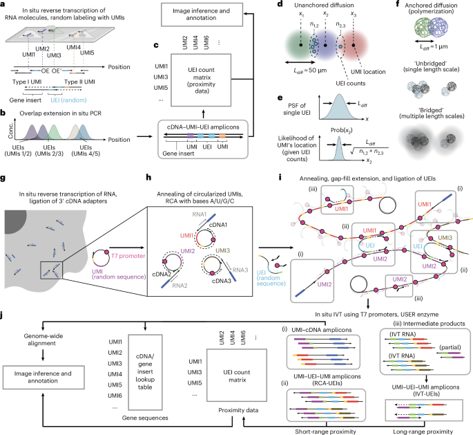
- DNA microscopy is an innovative technique that creates 3D spatial-genetic maps directly from biological tissues without relying on prior genetic or spatial facts.
- It functions by encoding molecular positions into DNA molecules and uses computational methods to reconstruct the specimen’s genetic image.
- Advances in this technology enable volumetric imaging of intact tissues, overcoming previous hurdles like thermal cycling challenges, computational scalability, and multi-scale data representation.
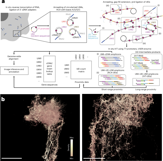
- Demonstrated on zebrafish embryos, it integrates genomic and morphological analysis at high resolution in 3D space.
Indian Opinion Analysis
DNA microscopy marks a breakthrough for scientific research, notably in developmental biology and disease studies. by integrating genomic mapping with spatial context at nucleotide-level precision,this technology has meaningful implications for understanding complex biological systems. For India’s growing biotechnology sector-already expanding through startups and collaborations-this advancement highlights future possibilities for indigenous adoption or development of similar techniques. Moreover, applying such innovations could strengthen India’s position in gene-editing research while contributing to global advances in personalized medicine and genomics-driven diagnostics.
Read MoreQuick Summary:
- Researchers developed a DNA microscopy methodology using two distinct Unique Molecular Identifiers (UMIs) to prevent interference.
- The method mixes rolling circle amplification (RCA) and in vitro transcription (IVT) for high spatial resolution of DNA interactions.
- This approach was validated using a zebrafish embryo model, enhancing spatial mapping through innovative biochemical techniques like proteinase K permeabilization.
- Computational methods including Geodesic Spectral Embeddings (GSE) were introduced to mathematically infer molecular coordinates from DNA microscopy data with enhanced efficiency.
- Benchmarking showed GSE effectively maps spatial genetic relationships in both 2D and 3D scenarios, improving upon previous algorithms.
Indian Opinion Analysis:
This study exemplifies advancements in genomic imaging technology that could complement existing sequencing techniques. For India, adopting such cutting-edge tools has potential implications for biomedical research, particularly when studying genetic diseases or biodiversity. The adaptability of this methodology could aid interdisciplinary research across bioinformatics and genomics fields. Investments in computational biology infrastructure might soon become essential as similar intricate technologies gain traction globally.
Read MoreQuick Summary
- Researchers applied advanced DNA microscopy techniques to spatially reconstruct biological specimens, including zebrafish embryos in 2D and 3D.
- The approach used Ground State embedding (GSE) for dimensionality reduction, improving resolution and scalability in constructing spatial genetic maps of UMIs (Unique Molecular Identifiers).
- Comparative analyses demonstrated the robustness of hierarchical GSE against undersampling artifacts, establishing resolution limits proportional to UEI counts per UMI.
- Zebrafish embryo imaging yielded reconstructions capturing structural patterns with median resolutions slightly above 1μm and confirmed gross morphology consistency across samples.
- Gene expression comparisons between DNA microscopy datasets and Stereo-seq identified similar enrichment trends along the anterior-posterior axis of zebrafish embryos using smoothed proximity-based mappings.
- Findings underscore DNA microscopy’s capacity for volumetric imaging without optical devices, weaving molecular connectivity into spatial data representations for diverse biological systems.
Indian Opinion Analysis
The study’s integration of GSE with molecular-level imaging provides a significant leap for India’s scientific community in decoding genetic architectures at increasingly precise scales. Scaling such methodologies allows researchers to explore genomic complexities more affordably than traditional light or electron microscopes while broadening accessibility across varied research institutions globally-including those focusing on non-model organisms indigenous to India like the Asiatic lion or Indian Bengal tiger species.With emphasis on reproducibility amidst detailed algorithmic frameworks tackling stochastic dispersion limits-broader applications lie ahead within medical genomics pipelines addressing localized diseases or neuron-mapping startups seeking heightened regional diagnostics potential acceleration pathways enhancing stronger trans-discipline-fluencyThe raw text provided is related to a technical research article on DNA microscopy and does not relate to India or fall within the scope of an indian news platform’s domain. Thus, it does not align with the task of summarizing news about India. Please provide relevant content related to Indian news, events, or topics.Quick Summary:
- The article discusses DNA microscopy as a novel imaging technique that generates spatio-genetic maps without the use of optical tools.
- It elaborates on mathematical modeling and image inference methods for analyzing experimental datasets, relying heavily on UMI (Unique Molecular Identifier) counts and matrix computations.
- Several computational approaches, including GSE (Geodesic Smoothing Embedding), are described to enhance dimensional reduction and improve accuracy in representing molecular spatial data.
- Issues surrounding resolution limits are explained using Gaussian approximation methods, highlighting challenges in precision due to varying UMI densities and diffusion properties.
Indian Opinion Analysis:
The advancements in DNA microscopy could have significant implications for India’s scientific community, particularly its biotechnology and genomics sectors. As an optics-free imaging technology, it has the potential to revolutionize biomedical research by enabling more efficient mapping of genetic interactions at a spatial level. However, implementing such high-end techniques would require ample investment into computational infrastructure for advanced data analysis-an area where India is emerging but still developing globally competitive capabilities. Encouraging collaboration between academic institutions and industries may help bridge technological gaps while tapping into the vast human resource pool of skilled researchers and bioinformaticians present in the country.
Read moreQuick Summary:
- the article delves into advanced computational methods, particularly hierarchical GSE (Generalized Spectral Embedding), for analyzing large datasets and handling uncertainty in complex systems.
- Emphasis is placed on the reconstruction of data through subgraph selection,linear interpolation of partial solutions,and reduction of noise using statistical regularization techniques.
- Applications mentioned include DNA microscopy datasets where iterative filtering was applied to address noise and overdispersion challenges.
- Additional methodologies involve Procrustes alignment for rigid alignment of spatial distributions and empirical quantile transformations to stabilize variance across data dimensions.
Indian Opinion Analysis:
The discussed techniques represent a significant stride in data science by tackling intricate computational challenges with precision-focused approaches like hierarchical GSE.For research institutes in India working on fields like biotech or big-data analytics (e.g., genomic studies), such methodologies can enhance the capability to deal with voluminous datasets effectively while ensuring accuracy. Moreover, the integration of these advancements into academic curriculums or innovative startups can propel India’s standing in cutting-edge tech solutions globally.


Related Posts
Stay Informed With the Latest & Most Important News
Previous Post
Next Post


Advertisement